Simulating with the MVS
The MVS can perform capacity as well as dispatch optimisations of a specific energy system. This means that both the capacity that is to be bought is optimised as well as the respective asset’s operation. To perform an energy system simulation, a multitude of input parameters is needed, which are described in link. They include economic parameters, technological parameters and project settings. Together they define all aspects of the energy system to be simulated and optimised. With this, the MVS builds an energy system model which is translated to an equation system which is to be solved. The MVS tries to minimise the annual costs of demand supply.
In this section, we want to provide you with all information needed to run your own optimisations. First we will explain the two input types, json and csv, and then how to make an energy system model out of your real local energy system configuration.
Input files
All input files need to be stored in a specifically formatted input folder. The path to the input folder is up to you.
There are two options to insert all input data – Json and CSV. These will be explained below.
Csv files: csv_elements folder
Usually a user, that is not using the MVS in combination with the EPA, will use CSV input files to define the local energy system, and respectively, the scenario.
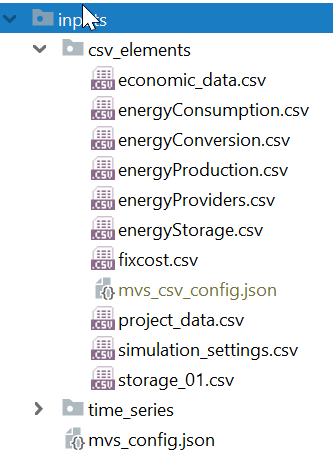
Specifically, the MVS will create a Json file (“mvs_csv_config.json”) from the provided input data, that works just like above described “mvs_config.json”. For that, each of the following files have to be present in the folder “csv_elements”:
economic_data.csv - Major economic parameters of the project
energyBusses.csv - Energy busses of the energy system to be simulated
energyConsumption.csv - Energy demands and paths to their time series as csv
energyConversion.csv - Conversion/transformer objects, eg. transformers, generators, heat pumps
energyProduction.csv - Act as energy “sources”, ie. PV or wind plants, with paths to their generation time series as csv
energyProviders.csv - Specifics of energy providers, ie. DSOs that are connected to the local energy system, including energy prices and feed-in tariffs
energyStorage.csv - List of energy storages of the energy system
storage_01.csv - Technical parameters of each energy system
fixcost.csv - fix project development/maintenance costs (should not be used currently)
simulation_settings.csv - Simulation settings, including start date and duration
project_data.csv - some generic project information
For easy set-up of your energy system, we have provided an empty input folder template as well here.
You can conveniently create a copy of this folder in your local path with the command (after having followed the installation steps) .. code:
mvs_create_input_template
A simple example system is setup with this input folder. When defining your energy system with this CSV files, please also refer to the definition of parameters that you can find here: stable / latest.
Please note that the allowed separators for csv files are located in src/constants.py under the CSV_SEPARATORS variable. Currently only [“,”, “;”, “&”] are allowed. Please note further that the column headers in the csv files need to be unique amongst all files.
Time series: time_series folder
As some parameters in the csv files link to a time series provided as a CSV, the folder “time_series” should be present in your input folder and provide all necessary input time series. This can include for example PV generation time series and demand time series.
The time series describing a non-dispatchable demand or when a time series defines an otherwise scalar value of a parameter (eg. energy price), the time series can have any absolute values.
For non-dispatchable sources, eg. the generation of a PV plant, you need to provide a specific time series (unit: kWh/kWp, etc.). For the latter, make sure that its values are between zero and one ([0, 1]).
Json file: mvs_config.json
In combination especially with the planned graphical user interface for the MVS (EPA), a json file will be used to store and provide all input data necessary to understand relation. The Json file itself is created by the EPA, ie. there are no manual changes. You can use a specific Json input file if you want to test a simulation that has been made public online, one test simulation, or as a developer that has knowingly edited the Json file.
As this requires to adhere to quite specific formatting rules, this can really only be recommended for advanced users.
There can only be a single Json file in your input folder. As some parameters in the Json file link to a time series provided as a CSV, the folder “time_series” should be present in your input folder, as clarified in the next section.
Defining an energy system
For defining your energy system you basically have to fill out the CSV sheets that are provided in the folder “csv_elements”. For each asset you want to add, you have to add a new column. If you do not have an asset of a specific type, simply leave the columns empty (but leave the columns with the parameter names and units).
The unit columns also tell you what type of information is required from you (string, boolean, number). In case of doubts, also consider the parameter list that is linked above. Do not delete any of the rows of the CSV´s – each parameter is needed for the simulation. There will also be warnings if you do so.
Example of simple energy systems
Input files of simple benchmarks (PV + battery + grid) scenarios can be found here
Building a model from assets and energy flows
Simulating an energy system with the MVS requires a certain level of abstraction. In general, as it is based on the programming framework oemof, it will depict the energy system only as linearized model. This allows for the quick computation of the optimal system sizing and approximate dispatch, but does not replace operational management.
The level of abstraction and system detail needed for an MVS simulation will be explained based on an exemplary local energy system. Let’s assume that we want to simulate an industrial site with some electrical demand, the grid connection, a battery as well as a PV plant. A schematic of such a system is shown below.
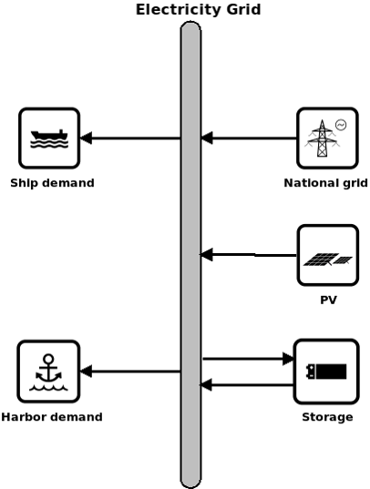
We can see that we have an electricity bus, to which all other components are connected, specifically demand external electricity supply and the local assets (battery and PV). However even though all those components belong to the same sector, their interconnection with the electricity bus or here the electricity grid could be detailed in the deeper manner.
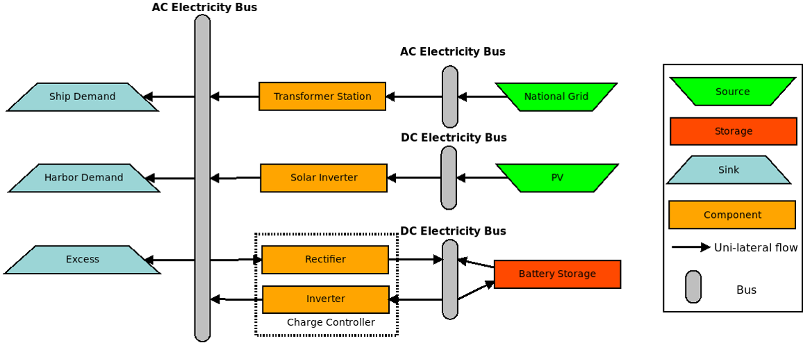
As such, in reality, the battery may be on an own DC electricity bus, which is either the separate from or identical to the DC bus of the PV plant. Both DC busses would have to be interconnected with the main electricity bus (AC) through an inverter, or in case of bi-directional flow for the battery with an rectifier as well.
Just like so, the DSO could either be only providing electricity also allowing feed in, or the demand may be split up into multiple demand profiles. This granularity of information would be something that the MVS model requires to properly depict the system behaviour and resulted optimal capacities and dispatch. The information fed into the MVS via the CSV’s would therefore define following components:
Ideally you scratch down the energy system you want to simulate with the above-mentioned granularity and only using sources, sinks, transformers and buses (meaning the oemof components). When interconnecting different assets make sure that you use the correct bus name in each of the CSV input files. The bus names are defined with input_direction and output_direction. If you interconnect your assets or buses incorrectly the system will still be built but the simulation terminated. If you’re not sure whether or not you build your system correctly change the parameter plot_networkx_graph in the simulation_settings to True. When executing the simulation, the MVS will now generate a rough graphic visualisation of your energy system. There, all components and buses should be part of a single system (i.e. linked to each other) - otherwise you misconfigured your energy system.
You need to be aware that you yourself have to make sure that the units you assign to your assets and energy flows make sense. The MVS does neither perform a logical check, nor does it transform units, eg. from MWh to kWh.
Adding a timeseries for a parameter
Sometimes you may want to define a parameter not as a scalar value but as a time series. This can for example happen for efficiencies (heat pump COP during the seasons), energy prices (currently only hourly resolution), or the state of charge (for example if you want to achieve a certain stage of charge of an FCEV at a certain point of time).
You can define a scalar as a time series in the csv input files (not applicable for energyConsumption.csv), by replacing the scalar value with following dictionary:
{‘file_name’: ‘your_file_name.csv’, ‘header’: ‘your_header’, ‘unit’: ‘your_unit’}
The feature was tested for following parameters:
energy_price
feedin_tariff
dispatch_price
efficiency
You can see an implemented example here, where the heat pump has a time-dependent efficiency:
unit |
heat_pump |
|
|---|---|---|
age_installed |
year |
0 |
development_costs |
currency |
0 |
specific_costs |
currency/kW |
7000 |
efficiency |
factor |
{‘file_name’: ‘cops_eers_test.csv’, ‘header’: ‘no_unit’, ‘unit’: ‘NA’} |
inflow_direction |
str |
Electricity |
installedCap |
kW |
0 |
label |
str |
Heat pump |
lifetime |
year |
20 |
specific_costs_om |
currency/kW/year |
0 |
dispatch_price |
currency/kWh |
0 |
optimizeCap |
bool |
True |
outflow_direction |
str |
Heat |
energyVector |
str |
Electricity |
type_oemof |
str |
transformer |
unit |
str |
kW |
The feature is tested with benchmark test test_benchmark_feature_parameters_as_timeseries().
Example input files, where at least one parameter is defined as a time series, can be found here:
First example: Defines the energy_price (file) of an energy provider as a time series
Second example: Defines the energy_price (file) of an energy provider and the efficiency of a diesel generator (file) as a time series.
Using multiple in- or output busses
Sometimes, you may also want to have multiple input- our output busses connected to a component. This is for example the case if you want to implement an electrolyzer with a transformer, and want to track water consumption at the same time as you want to track electricity consumption.
You can define this, again, in the csv´s. Here, you would insert a list of your parameters instead of the scalar value of a parameter:
[0.99, 0.98]
Would be an example of a transformer with two efficiencies.
You can also wrap multiple inputs/outputs with scalars that are defined as efficiencies. For that, you define one or multiple of the parameters within the list with the above introduced dictionary:
[0.99, {‘value’: {‘file_name’: ‘your_file_name.csv’, ‘header’: ‘your_header’}, ‘unit’: ‘your_unit’}]
If you define an output- or input flow with with a list, you also have to define related parameters as a list. So, for example, if you define the input direction as a list for an energyConsumption asset, you need to define the efficiencies and dispatch_price costs as a list as well.
You can see an implemented example here, where the heat pump has a time-dependent efficiency:
unit |
electrolyser |
|
|---|---|---|
age_installed |
year |
3 |
development_costs |
currency |
0 |
specific_costs |
currency/kW |
1500 |
efficiency |
factor |
[0.01923,0.28845] |
inflow_direction |
str |
[MicroGrid,Water] |
installedCap |
kW |
0 |
label |
str |
Electrolyser |
lifetime |
year |
20 |
specific_costs_om |
currency/kW/year |
75 |
dispatch_price |
currency/kWh |
[0,0.0038] |
optimizeCap |
bool |
True |
outflow_direction |
str |
Local H2 grid |
energyVector |
str |
Electricity |
type_oemof |
str |
transformer |
unit |
str |
kW |
The features were integrated with Pull Request #63. For more information, you might also reference following issues: