Outputs of the MVS simulation
System schematic
plot_networkx_graph
Optimal capacities
Cost data
Net present cost
The Net present cost (NPC) is the present value of all the costs associated with installation, operation, maintenance and replacement of energy technologies comprising the sector-coupled system over the project lifetime, minus the present value of all the revenues that it earns over the project lifetime. The capital recovery factor (CRF) is used to calculate the present value of the cash flows.
** The content of this section was copied from the conference paper handed in to CIRED 2020**
Levelized costs of energy (LCOE)
As a sector-coupled system connects energy vectors, not the costs associated to each individual energy carrier but the overall energy costs should be minimized. Therefore, we propose a new KPI: The levelized costs of energy (LCOEnergy) aggregates the costs for energy supply and distributes them over the total energy demand supplied, which is calculated by weighting the energy carriers by their energy content. To determine the weighting factors of the different energy carriers, we reference the method of gasoline gallon equivalent (GGE) [12], which enables the comparison of alternative fuels. Instead of comparing the energy carriers of an MES to gasoline, we rebase the factors introduced in [12] onto the energy carrier electricity, thus proposing a unit Electricity Equivalent (ElEq). The necessary weights are summarized in Table 1. With this, we propose to calculate LCOEnergy based on the annual energy demand and the systems annuity, calculated with the CRF, as follows:
Specific electricity supply costs, eg. levelized costs of electricity (LCOElectricity) are a common KPI that can be compared to local prices or generation costs. As in a sector-coupled system the investments cannot be clearly distinguished into sectors, we propose to calculate the levelized costs of energy carriers by distributing the costs relative to supplied demand. The LCOElectricity are then calculated with:
** The content of this section was copied from the conference paper handed in to CIRED 2020**
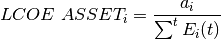
Levelized Cost of Energy of Asset (LCOE ASSET)
This KPI measures the cost of generating 1 kWh for each asset in the system. It can be used to assess and compare the available alternative methods of energy production. The levelized cost of energy of an asset (LCOE ASSET) is usually obtained by looking at the lifetime costs of building and operating the asset per unit of total energy throughput of an asset over the assumed lifetime [currency/kWh].
Since not all assets are production assets, the MVS distinguishes between the type of assets.
For assets in energyConversion and energyProduction the MVS calculates the LCOE ASSET
by dividing the total annuity  of the asset
  by the total flow
  .
.
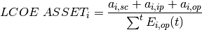
For assets in energyStorage, the MVS sums the annuity for storage capacity  , input power $a_{i,ip}$ and output power
  and divides it by the output power total flow
  .
.
If the total flow is 0 in any of the previous cases, then the LCOE ASSET is set to None.

For assets in energyConsumption, the MVS outputs 0 for the LCOE ASSET.

Technical data
Energy flows (aggregated) per asset
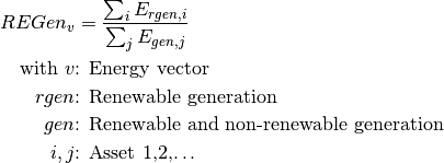
Renewable share of local generation (REGen)
The renewable share of local generation describes how much of the energy generated locally is produced from renewable sources. It does not take into account the consumption from energy providers.
The renewable share of local generation for each sector does not utilize energy carrier weighting but has a limited, single-vector view:
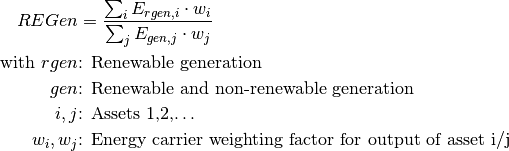
For the system-wide share of local renewable generation, energy carrier weighting is used:
- Example
An energy system is composed of a heat and an electricity side. Following are the energy flows:
100 kWh from a local PV plant
0 kWh local generation for the heat side
This results in:
A single-vector renewable share of local generation of 0% for the heat sector.
A single-vector renewable share of local generation of 100% for the electricity sector.
A system-wide renewable share of local generation of 100%.
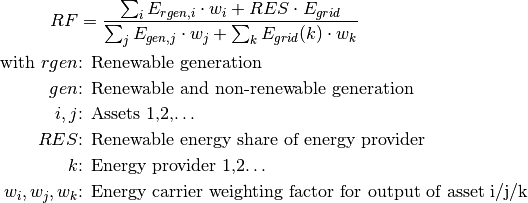
Renewable factor (RF)
Describes the share of the energy influx to the local energy system that is provided from renewable sources. This includes both local generation as well as consumption from energy providers.
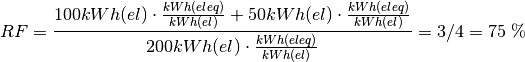
- Example
An energy system is composed of a heat and an electricity side. Following are the energy flows:
100 kWh from a local PV plant
0 kWh local generation for the heat side
100 kWh consumption from the electricity provider, who has a renewable factor of 50%
Again, the heat sector would have a renewable factor of 0% when considered separately, and the electricity side would have an renewable factor of 75%. This results in a system-wide renewable share of:
The renewable factor can, just like the Renewable share of local generation (REGen) not indicate how much renewable energy is used in each of the sectors. In the future, it may be possible to dive into this together with the degree of sector-coupling.
Emissions
The total emissions of the MES in question are calculated with all aggregated energy flows from the generation assets including energy providers and their subsequent emission factor:
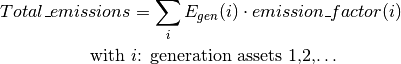
The emissions of each generation asset and provider are also calculated and displayed separately in the outputs of MVS.
Additionally, the specific emissions per electricity equivalent of the MES are calculated in  :
:
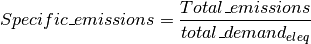
Emissions can be of different nature: CO2 emissions, CO2 equivalents, greenhouse gases, …
Currently the emissions do not include life cycle emissions of energy conversion or storage assets, nor are they calculated separately for the energy sectors. For the latter, it arises the problem of the assignment of assets to sectors. E.g. emissions caused by an electrolyser would be counted to the electricity sector although you might want to count it for the H2 sector, as the purpose of the electrolyser is to feed the H2 sector. Therefore, we will have to verify whether or not we can apply the energy carrier weighting also for this KPI.
Degree of sector-coupling (DSC)
While a MES includes multiple energy carriers, this fact does not define how strongly interconnected its sectors are. To measure this, we propose to compare the energy flows in between the sectors to the energy demand supplied:
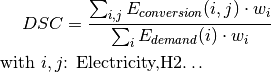
** The content of this section was copied from the conference paper handed in to CIRED 2020**
Onsite energy fraction (OEF)
Onsite energy fraction is also referred to as self-consumption. It describes the fraction of all locally generated energy that is consumed by the system itself. (see [1] and [2]).
An OEF close to zero shows that only a very small amount of locally generated energy is consumed by the system itself. It is at the same time an indicator that a large amount is fed into the grid instead. A OEF close to one shows that almost all locally produced energy is consumed by the system itself. Notice that the feed into the grid can only be positive.
![OEF &=\frac{\sum_{i} {E_{generation} (i) \cdot w_i} - E_{gridfeedin}(i) \cdot w_i}{\sum_{i} {E_{generation} (i) \cdot w_i}}
&OEF \epsilon \text{[0,1]}](_images/math/5f95e8b3e07ae34207f5d58a25b365489364652d.png)
Onsite energy matching (OEM)
The onsite energy matching is also referred to as “self-sufficiency”. It describes the fraction of the total demand that can be covered by the locally generated energy (see [1] and [2]). Notice that the feed into the grid should only be positive.
An OEM close to zero shows that very little of the demand can be covered by locally produced energy. Am OEM close to one shows that almost all of the demand can be covered with locally generated energy. Per definition OEM cannot be greater than 1 because the excess generated energy would automatically be fed into the grid or an excess sink.
![OEM &=\frac{\sum_{i} {E_{generation} (i) \cdot w_i} - E_{gridfeedin}(i) \cdot w_i - E_{excess}(i) \cdot w_i}{\sum_i {E_{demand} (i) \cdot w_i}}
&OEM \epsilon \text{[0,1]}](_images/math/3943ac7bc53181bcd8c18a2cc4804f1bed81f701.png)
Degree of autonomy (DA)
The degree of autonomy describes the overall energy consumed minus the energy consumed from the grid divided by the overall energy consumed. Adapted from this definition [3].
A degree of autonomy close to zero shows high dependence on the grid operator, while a degree of autonomy of one represents an autonomous system. Note that this key parameter indicator does not take into account the outflow from the system to the grid operator (also called feedin). As above, we apply a weighting based on Electricity Equivalent.

Degree of net zero energy (NZE)
The degree of net zero energy describes the ability of an energy system to provide its aggregated annual demand though local sources. For that, the balance between local generation as well as consumption from and feed-in towards the energy provider is compared. In a net zero energy system, demand can be supplied by energy import, but then local energy generation must provide an equally high energy export of energy in the course of the year. In a plus energy system, the export exceeds the import, while local generation can supply all demand (from an aggregated perspective). To calculate the degree of NZE, the margin between grid feed-in and grid consumption is compared to the overall demand.
Some definitions of NZE systems require that the local demand is solely covered by locally generated renewable energy. In MVS this is not the case - all locally generated energy is taken into consideration. For information about the share of renewables in the local energy system checkout Renewable share of local generation (REGen).
A degree of NZE lower 1 shows that the energy system can not reach a net zero balance, and indicates by how much it fails to do so, while a degree of NZE of 1 represents a net zero energy system and a degree of NZE higher 1 a plus-energy system.
As above, we apply a weighting based on Electricity Equivalent.

Automatic Report
MVS has a feature to automatically generate a PDF report that contains the main elements from the input data as well as the simulation results’ data. The report can also be viewed as a web app on the browser, which provides some interactivity.
MVS version number, the branch ID and the simulation date are provided as well in the report, under the MVS logo. A commit hash number is provided at the end of the report in order to prevent the erroneous comparing results from simulations using different versions.
It includes several tables with project data, simulation settings, the various demands supplied by the user, the various components of the system and the optimization results such as the energy flows and the costs. The report also provides several plots which help to visualize the flows and costs.
Please, refer to the report section for more information on how to setup and use this feature, or type
mvs_report -h
in your terminal or command line.