Limitations
When running simulations with the MVS, there are certain peculiarities to be aware of. The peculiarities can be considered as limitations, some of which are merely model assumptions and others are drawbacks of the model. A number of those are inherited due to the nature of the MVS and its underlying modules. The following table (Limitations) lists the MVS limitations based on their type.
Infeasible bi-directional flow in one timestep
- Limitation:
It is not possible to model two flows in opposite directions during the same time step.
- Reason:
The MVS is based on the python library oemof-solph. Its generic components are used to set up the energy system. As a ground rule, the components of oemof-solph are unidirectional. This means that for an asset that is bidirectional two transformer objects have to be used. Examples for this are:
Physical bi-directional assets, eg. inverters
Logical bi-directional assets, eg. consumption from the grid and feed-in to the grid
To achieve the real-life constraint one flow has to be zero when the other is larger zero, one would have to implement following relation:
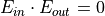
However, this relation creates a non-linear problem and can not be implemented in oemof-solph.
- Implications:
This limitation means that the MVS might result in infeasible dispatch of assets. For instance, a bus might be supplied by a rectifier and itself supplying an inverter at the same time step t, which cannot logically happen if these assets are part of one physical bi-directional inverter. Another case that could occur is feeding the grid and consuming from it at the same time t.
Under certain conditions, including excess generation as well as dispatch costs of zero, the infeasible dispatch can also be observed for batteries and result in a parallel charge and discharge of the battery. If this occurs, a solution may be to set a marginal dispatch cost of battery charge.
Simplified linear component models
- Limitation:
The MVS simplifies the component model of some assets.
Generators have an efficiency that is not load-dependent
Storage have a charging efficiency that is not SOC-dependent
Turbines are implemented without ramp rates
- Reason:
The MVS is based oemof-solph python library and uses its generic components to set up an energy system. Transformers and storages cannot have variable efficiencies, because otherwise the system of equation to solve would not be linear.
- Implications:
Simplifying the implementation of some component specifications can be beneficial for the ease of the model, however, it contributes to the lack of realism and might result in less accurate values. The MVS trades off the decreased level of detail for a quick evaluation of its scenarios, which are often only used for a pre-feasibility analysis.
No degradation of efficiencies over a component lifetime
- Limitation:
The MVS does not degrade the efficiencies of assets over the lifetime of the project, eg. in the case of production assets like PV panels.
- Reason:
The simulation of the MVS is only based on a single reference year, and it is not possible to take into account multi-year degradation of asset efficiency.
- Implications:
This results in an overestimation of the energy generated by the asset, which implies that the calculation of some other results might also be overestimated (e.g. overestimation of feed-in energy). The user can circumvent this by applying a degradation factor manually to the generation time series used as an input for the MVS.
Perfect foresight
- Limitation:
The optimal solution of the energy system is based on perfect foresight.
- Reason:
As the MVS and thus oemof-solph, which is handling the energy system model, know the generation and demand profiles for the whole simulation time and solve the optimization problem based on a linear equation system, the solver knows their dispatch for certain, whereas in reality the generation and demand could only be forecasted.
- Implications:
The perfect foresight can lead to suspicious dispatch of assets, for example charging of a battery right before a (in real-life) random blackout occurs. The systems optimized with the MVS therefore, represent their optimal potential, which in reality could not be reached. The MVS has thus a tendency to underestimate the needed battery capacity or the minimal state of charge for backup purposes, and also designs the PV system and backup power according to perfect forecasts. In reality, operational margins would need to be considered.
Optimization precision
- Limitation:
Marginal capacities and flows below a threshold of 10^-6 are rounded to zero.
- Reason:
The MVS makes use of the open energy modelling framework (oemof) by using oemof-solph. For the MVS, we use the cbc-solver with a ratioGap=0.03. This influences the precision of the optimized decision variables, ie. the optimized capacities as well as the dispatch of the assets.
In some cases the dispatch and capacities vary around 0 with fluctuations of the order of floating point precision (well below <10e-6), thus resulting sometimes in marginal fluctuations dispatch or capacities around 0. When calculating KPI from these decision variables, the results can be nonsensical, for example leading to SoC curves with negative values or values far above the viable value 1.
As the reason for these inconsistencies is known, the MVS enforces the capacities and dispatch of to be above 10e-6, ie. all capacities or flows smaller than that are automatically set to zero. This is applied to absolute values, so that irregular (and incorrect) values for decision variables can still be detected.
- Implications:
If your energy system has demand or resource profiles that include marginal values below the threshold of 10^-6, the MVS will not result in appropriate results. For example, that means that if you have an energy system with usually is measured in MW but one demand is in the W range, the dispatch of assets serving this minor demand is not displayed correctly. Please consider using kW or even W as a base unit then.
Extension of KPIs necessary
- Limitation:
Some important KPIs usually required by developers are currently not implemented within the MVS:
Internal rate of return (IRR)
Payback period
Return on equity (ROE),
- Reason:
The MVS tool is a work in progress and this can still be addressed in the future.
- Implications:
The absence of such indicators might affect decision-making.
Random excess energy distribution
- Limitation:
There is random excess distribution between the feed-in sink and the excess sink when no feed-in-tariff is assumed in the system.
- Reason:
Since there is no feed-in-tariff to benefit from, the MVS randomly distributes the excess energy between the feed-in and excess sinks. As such, the distribution of excess energy changes when running several simulations for the same input files.
- Implications:
On the first glance, the distribution of excess energy onto both feed-in sink and excess sink may seem off to the end-user. Other than these inconveniences, there are no real implications that affect the capacity and dispatch optimization. When a degree of self-supply and self-consumption is defined, the limitation might tarnish these results.
Renewable energy share definition relative to energy carriers
- Limitation:
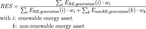
The current renewable energy share depends on the share of renewable energy production assets directly feeding the load. The equation to calculate the share also includes the energy carrier rating as described here below:
- Reason:
The MVS tool is a work in progress and this can still be addressed in the future.
- Implications:
This might result in different values when comparing them to other models. Another way to calculate it is by considering the share of energy consumption supplied from renewable sources.
Energy carrier weighting
- Limitation:
The MVS assumes a usable energy content rating for every energy carrier. The current version assumes that 1 kWh thermal is equivalent to 1 kWh electricity.
- Reason:
This is an approach that the MVS currently uses.
- Implications:
By weighing the energy carriers according to their energy content (Gasoline Gallon Equivalent (GGE)), the MVS might result in values that can’t be directly assessed. Those ratings affect the calculation of the levelized cost of the energy carriers, but also the minimum renewable energy share constraint.
Events of energy shortage or grid interruption cannot be modelled
- Limitation:
The MVS assumes no shortage or grid interruption in the system.
- Reason:
The aim of the MVS does not cover this scenario.
- Implications:
Electricity shortages due to power cuts might happen in real life and the MVS currently omits this scenario. If a system is self-sufficient but relies on grid-connected PV systems, the latter stop feeding the load if any power cuts occur and the battery storage systems might not be enough to serve the load thus resulting energy shortage.
Need to model one technical unit with two transformer assets
- Limitation:
Two transformer objects representing one technical unit in real life are currently unlinked in terms of capacity and attributed costs.
- Reason:
The MVS uses oemof-solph’s generic components which are unidirectional so for a bidirectional asset,
two transformer objects have to be used.
- Implications:
Since only one input is allowed, such technical units are modelled as two separate transformers that are currently unlinked in the MVS (e.g., hybrid inverter, heat pump, distribution transformer, etc.). This raises a difficulty to define costs in the input data. It also results in two optimized capacities for one logical unit.
This limitation can be addressed with a constraint which links both capacities of one logical unit, and therefore solves both the problem to attribute costs and the previously differing capacities.